Introduction
In this post, I will scrape the 2018 State of the State Addresses (SoSAs), convert the speeches into a dataframe of words counts with the rows representing the speeches and the columns representing the words. This type of dataframe is known as document term matrix (dtm). I will also perform some exploratory analysis of the constructed dataset.
Every year, at the beginning of the year, most U.S governors present their visions for their states in their SoSAs. The speech is meant, for the governor, to layout her vision for the state, and the means for achieving the vision. It is meant to present the governor’ legislative agenda and her proposed budget. It is arguably the governor most important speech of the year. Chiefly, the governor uses the speech to rally supports for her agenda. Thus, given its importance for understanding the state agenda, it may be useful to statistically explore the differences between governors in terms of their words choices. To do so, we need to scrape the data first.
Scraping the speeches
The web is the primary source for accessing the SoSAs. When we are interested in a few texts, it is easy to locate the links of the speeches, then copy the texts. However, copying and pasting becomes tedious when we need to collect dozens of speeches. Moreover, some of the text are in pdf format, and copying pdf files is sometimes not a trivial task. Therefore, we might find it more efficient to write a program that will grab the texts, for us, from the web. This task is generally referred as web scraping.
Getting the web links of the speeches
To scrape the data (or the texts), we first need to get the web links of the texts. Luckily, the web links of the 2018 SoSAs can be found here. The code below scrapes the table of the web links.
# required packages
library(pdftools) # needed to download and extract text from .pdf files
library(rvest) # needed to download and extract text from html files
library(stringr) # needed for string manipulation
library(dplyr) # needed for dataframe manipulation
library(tm) # needed for text mining


# get the table of governors and the links of the speeches
# sp stands for speeches
sp_url <- "https://www.multistate.us/2018-state-of-the-state-addresses-0"
sp_webpage <- read_html(sp_url)
sp_tabl <- sp_webpage %>%
  html_nodes("table") %>%
  .[[1]] %>%
  html_table(header = 1)

Party <- c("R", "I", "R", "R", "D", "D", "D", "D", "R", "R",
           "D", "R", "R", "R", "R", "R", "R", "D", "R", "R",
           "R", "R", "D", "R", "R", "D", "R", "R", "R", "R",
           "R", "D", "D", "R", "R", "R", "D", "D", "D", "R",
           "R", "R", "R", "R", "R", "D", "D", "R", "R", "R")

sp_tabl$Party <- Party

sp_tabl <- sp_tabl %>%
  filter(Date != 'None')
links <- sp_webpage %>%
  html_nodes(xpath = '//table/..//a') %>%
  html_attr('href')
sp_tabl$Links <- links
sp_tabl <- sp_tabl %>%
  filter(State != 'Texas') # Texas’s file is not a speech. So remove it.
Below is the table of the web links and some metadata of the speeches
library(knitr)
library(kableExtra)
kable(head(sp_tabl[, -4]), "html") %>%
kable_styling(bootstrap_options = "striped", full_width = F)| State | Governor | Date | Party | Links |
|---|---|---|---|---|
| Alabama | Kay Ivey | 1/9/18 | R | https://governor.alabama.gov/remarks-speeches/2018-state-of-the-state-address/ |
| Alaska | Bill Walker | 1/18/18 | I | https://gov.alaska.gov/wp-content/uploads/sites/5/2018-State-of-the-State.pdf |
| Arizona | Doug Ducey | 1/8/18 | R | https://azgovernor.gov/governor/news/2018/01/arizona-state-state-2018 |
| Arkansas | Asa Hutchinson | 2/12/18 | R | https://governor.arkansas.gov/speeches/detail/state-of-the-state |
| California | Jerry Brown | 1/25/18 | D | https://www.gov.ca.gov/news.php?id=20150 |
| Colorado | John Hickenlooper | 1/11/18 | D | https://www.colorado.gov/governor/sites/default/files/2018_state_of_the_state_speech.pdf |
Downloading and extracting the texts
rvest is a popular R package for scraping html files. However, some of the files we are scraping are in pdf format. Therefore, we will have to supplement rvest with the pdftools package to scrape both the .pdf and .html files. To do so, we write a loop that checks whether the file to download is a .pdf or not. If the file is a pdf, then the pdftools’ functions are used to download the file and extract its text. If the file is not a pdf, then we use rvest’s functions to download the file and extract its text. Unfortunately, some of the links are dead, others do not link to .pdf nor .html files. So, we use tryCatch to prevent the loop from crashing, just because the code cannot download a file. The following code does the trick.
# Download the files, then extract the text data

sp_number = 0
missing <- NULL
for (url in sp_tabl$Links) {
  sp_number = sp_number + 1
  has_a_pdf <- str_detect(string = url, pattern = '.pdf')
  if(has_a_pdf){ # scrape text from .pdf files
    text <- tryCatch(pdf_text(url),
                     error = function(e) e)
    if(inherits(text, "error")){
      missing <- c(missing, sp_number)
      next
    }
    text <- paste(unlist(strsplit(text, "\n")), collapse = "")
    path <- paste0('speeches/', sp_tabl$State[sp_number], ".txt")
    fileConn<-file(path)
    writeLines(text, fileConn)
    close(fileConn)
  } else{  # scrape text from html files
    text <- tryCatch(read_html(url), # to prevent errors from crashing the loop
                     error = function(e) e)
    if(inherits(text, "error")){
      missing <- c(missing, sp_number)
      next
    }
    text <- text %>%
      html_nodes(xpath = '//p') %>%
      html_text()
    path <- paste0('speeches/', sp_tabl$State[sp_number], ".txt")
    fileConn<-file(path)
    writeLines(text, fileConn)
    close(fileConn)
  }
  Sys.sleep(5) # slows down the files request.
}
The code above downloads the files, extracts the text, and saves the files in the directory provided. I saved the texts in a folder named speeches. A quick check of the .txt files in the speeches directory shows that a couple of files are empty. That may be due to several possible reasons. (1) some files are not .pdf, nor .html (Utah). (2) A file may be a .pdf but the link does not contain a pdf so it fails to be treated as pdf (Wyoming). (3) Others files have unusual html tags for the text (West Virginia). In sum, inconsistency is a problem when scraping data from several sources. And, in practice, we have to iterate the process to detect the possible inconsistencies and adjust the code accordingly. For further notes on web scraping with R, see this, this, or this.
Transforming the text documents into a matrix of words count per document
The tm package is one of the most popular R packages for text mining. Here, the goal is to convert the text documents into a matrix of words counts, where each row represents a speech and each column represents a word; a cell represents the number of times a particular word was used in a particular speech. Also, it is customary to pre-process the data before analysis; that is, depending on the type of analysis, some words may be considered useless, and removed from the dataset. Combining certains words may be warranted because they convey a single idea (for instance, education, educational covey the same idea), so we stem the words to avoid such words being considered as two separate words. For more on pre-processing, see page 4 of thistutorial. It should be noted that for some analyses, the small words (or transition words) may be the most important words (for example, in stylometrics, or authorship attribution).
# Convert text data into a table of words counts per document


MyDocuments <- DirSource("speeches/") #path for documents
MyCorpus <- Corpus(MyDocuments, readerControl=list(reader=readPlain)) #load in documents

f <- content_transformer(function(x, pattern) gsub(pattern, " ", x))
MyCorpus <- tm_map(MyCorpus, f, "[^[:alnum:]]") # Remove anything that is not alphanumeric
MyCorpus <- tm_map(MyCorpus, content_transformer(tolower))
MyCorpus <- tm_map(MyCorpus, removeWords, stopwords('english'))
MyCorpus <- tm_map(MyCorpus, stripWhitespace)
MyCorpus <- tm_map(MyCorpus, removePunctuation)
MyCorpus <- tm_map(MyCorpus, removeNumbers)


dtm <- DocumentTermMatrix(MyCorpus,
                          control = list(wordLengths = c(4, Inf), stemming = TRUE))
Sp_dtm <- dtm %>% removeSparseTerms(sparse=0.75) # Drop words that are present in less than 25% of the documents
#dim(Sp_dtm) # inspect the dimension of the data set
Sp_dtm_df <- as.data.frame(as.matrix(Sp_dtm)) # Convert table into a dataframe for ease of data manipulation
row_sums <- rowSums(Sp_dtm_df)
Sp_dtm_df$Party <- sp_tabl$Party
Sp_dtm_df$row_sums <- row_sums

Sp_dtm_df <- Sp_dtm_df %>%
  subset(row_sums > 100) # to remove empty (or very short) documents
Sp_dtm_df$row_sums = NULL
Overall, we get a dataframe of 42 rows (i.e. documents) and 906 columns (i.e. words); with the last column being the party affiliation of the governor. This dataframe can now be used to perform statistical analyses.
Performing statistical analysis of the words counts
Barplots of a selected list of words
Barplots are useful for exploring, graphically, count data. Below, we explore the top 20 most used words in all the speeches.
library(ggplot2) # needed for graphs
words_freq <- colSums(Sp_dtm_df[ ,-length(Sp_dtm_df)])
words_freq <- data.frame(words = names(words_freq),
                         freq = unname(words_freq))
words_freq <- words_freq[order(words_freq$freq, decreasing = TRUE),]


p <- ggplot(data = words_freq[1:20, ], aes(x=words, y=freq)) +
  geom_bar(stat="identity", fill="steelblue")
p + coord_flip()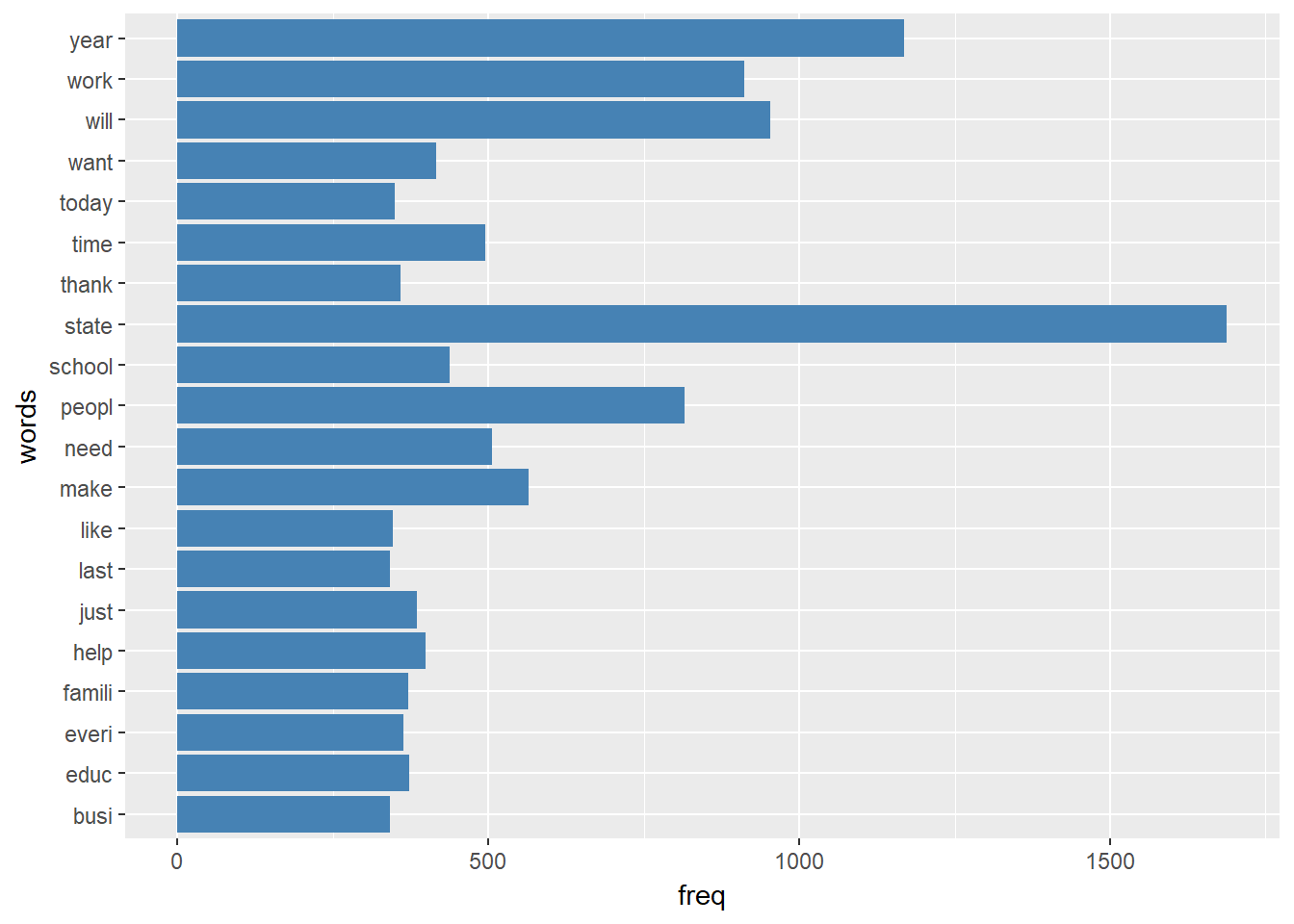
From the barplot, the most used words in the speeches are state, year, and will. Among the top twenty words are: School, Education, Business, and work.
Let’s select a few words, and compare the words relative frequencies by party affiliation. The words selected are: Education, Health, Budget, Economy, and Business. The stemming function did not do a good job. It was meant to convert words such as economy, economical into their root words. But, that did not happen. We will do it manually.
Sp_dtm_df$econom <- Sp_dtm_df$econom + Sp_dtm_df$economi
Sp_dtm_df$economi <- NULL
Sp_dtm_df$health <- Sp_dtm_df$health + Sp_dtm_df$healthi + Sp_dtm_df$healthcar
Sp_dtm_df$healthi <- NULL
Sp_dtm_df$healthcar <- NULL
Now, let’s select the words of interest, and explore them using a barplot.
selected_words <- Sp_dtm_df[, c("budget", "busi", "econom", "educ", "health", "Party")]

selected_words_D <- colSums(selected_words[selected_words$Party == "D" ,-length(selected_words)])
selected_words_D <- data.frame(words = names(selected_words_D),
                         freq = unname(selected_words_D)/sum(unname(selected_words_D)))
selected_words_D$party <- rep("D", 5)

selected_words_R <- colSums(selected_words[selected_words$Party == "R" ,-length(selected_words)])
selected_words_R <- data.frame(words = names(selected_words_R),
                         freq = unname(selected_words_R)/sum(unname(selected_words_R)))
selected_words_R$party <- rep("R", 5)

sel_word_D_R <- rbind(selected_words_D, selected_words_R)

p_DR <- ggplot(data = sel_word_D_R, aes(x=words, y=freq, fill = party)) +
  geom_bar(stat="identity", position=position_dodge())
p_DR + scale_fill_manual(values = c('blue','red')) +
  coord_flip()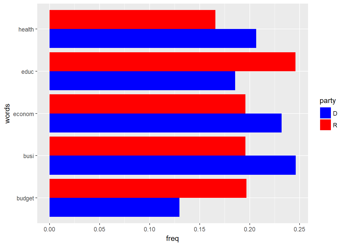
The barplot shows that, relatively, Democrats have used the words health, economy, and business more often than Republicans. The Republicans have used the words education and budget more often than the Democrats.
An alternative way to look at the words frequencies is to use a wordcloud. We will do so first, for all governors, then by party affiliation. Before that, we remove the words state, will, and year from the data. I am assuming that they are not important since they are so common in all speeches.
words_freq <- words_freq[words_freq$freq <= 900, ]
# or
Sp_dtm_df = subset(Sp_dtm_df, select = - c(state, will, year))
library("wordcloud")
library("RColorBrewer")
set.seed(4444) # needed to reproduce the exact same wordcloud
wordcloud(words = words_freq$words, freq = words_freq$freq, min.freq = 1,
max.words=350, random.order=FALSE, rot.per=0.35,
colors=brewer.pal(8, "Dark2"))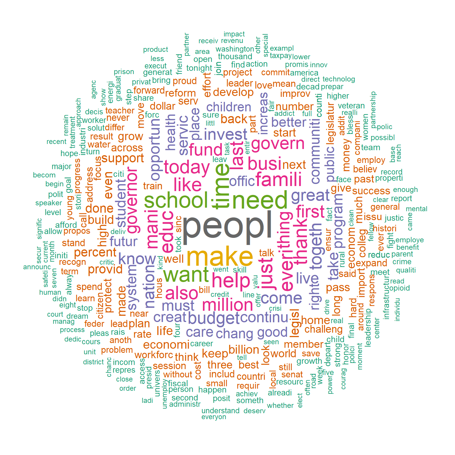
The wordcloud above indicates that people, education, health, business, family, budget are all prominent words in the speeches. Let’s look at the wordcloud by party affiliation (Democrats vs. Republicans).
dem_freq <- colSums(Sp_dtm_df[Sp_dtm_df$Party == "D",-length(Sp_dtm_df)])
rep_freq <- colSums(Sp_dtm_df[Sp_dtm_df$Party == "R",-length(Sp_dtm_df)])
comp_data <- data.frame(Democrats = unname(dem_freq)/sum(unname(dem_freq)),
                        Republicans = unname(rep_freq)/sum(unname(rep_freq)))
row.names(comp_data) <- names(dem_freq)
#comp_data <- round(comp_data*1000, 0)
comparison.cloud(comp_data,max.words=250,random.order=FALSE, colors = c("blue", "red"))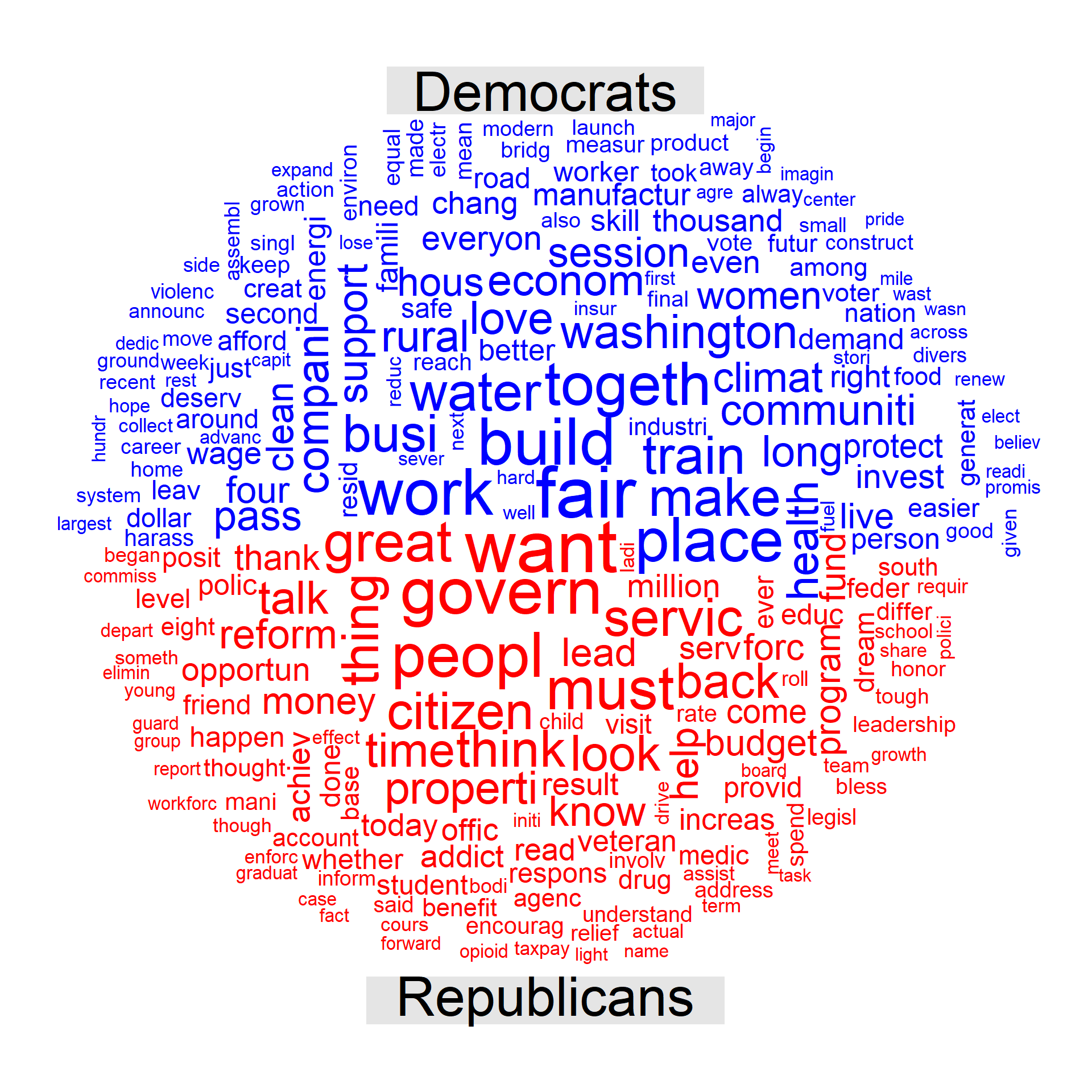
Clearly, Democrats and Republicans governors focused on different words during their 2018 SoSAs. Paradoxically, while Democrates used words related to the economy (fair, build, business, work, train) more often, Republicans used more words related to the state (govern, people, citizen, service, reform). There are much more differences that we can highlight, based on this wordcloud. What other differences can you highlight? I leave that to you.
Conclusion
This post has presented the steps from collecting text data from the web to exploring the data. Given that more data are found online these days, web scraping is certainly a valuable skill for data analytics. Converting the text data into a matrix of words counts allows us to perform traditional data exploration. Additional exploratory tools (such as wordcloud) designed for the particular case of text data exists. In this post, we went through introductory level tools of text analytics. Text analytics is an exciting branch of statistics (or machine learning if you will). In my opinion, text analytics is probably one of the most effective ways to learn data analysis, since nothing in text analytics is trivial, and exploratory analysis (and therefore human judgement) is paramount. This post is getting too long. Let’s leave it here. Feel free to leave your comments below!